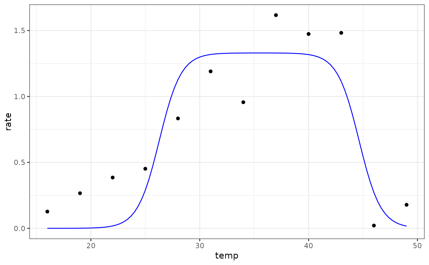
Ashrafi III model for fitting thermal performance curves
Value
a numeric vector of rate values based on the temperatures and parameter values provided to the function
Details
Equation: $$rate = \frac{1}{(a + b \cdot exp^{temp} + d \cdot exp^{-temp})}$$
Start values in get_start_vals are derived from the data or sensible values from the literature.
Limits in get_lower_lims and get_upper_lims are derived from the data or based extreme values that are unlikely to occur in ecological settings.
References
Ashrafi, R. et al. Broad thermal tolerance is negatively correlated with virulence in an opportunistic bacterial pathogen. Evolutionary Applications 11, 1700–1714 (2018).
Examples
# load in ggplot
library(ggplot2)

# subset for the first TPC curve
data('chlorella_tpc')
d <- subset(chlorella_tpc, curve_id == 1)

# get start values and fit model
start_vals <- get_start_vals(d$temp, d$rate, model_name = 'ashrafi3_2018')
# fit model
mod <- nls.multstart::nls_multstart(rate~ashrafi3_2018(temp = temp, a, b, c),
data = d,
iter = c(4,4,4),
start_lower = start_vals - 10,
start_upper = start_vals + 10,
lower = get_lower_lims(d$temp, d$rate, model_name = 'ashrafi3_2018'),
upper = get_upper_lims(d$temp, d$rate, model_name = 'ashrafi3_2018'),
supp_errors = 'Y',
convergence_count = FALSE)

# look at model fit
summary(mod)
#>
#> Formula: rate ~ ashrafi3_2018(temp = temp, a, b, c)
#>
#> Parameters:
#>    Estimate Std. Error t value Pr(>|t|)
#> a 7.518e-01  8.146e-02   9.229 6.95e-06 ***
#> b 3.090e-20  3.406e-20   0.907    0.388
#> c 1.949e+11  2.129e+11   0.915    0.384
#> ---
#> Signif. codes:  0 ‘***’ 0.001 ‘**’ 0.01 ‘*’ 0.05 ‘.’ 0.1 ‘ ’ 1
#>
#> Residual standard error: 0.3022 on 9 degrees of freedom
#>
#> Number of iterations till stop: 91
#> Achieved convergence tolerance: 1.49e-08
#> Reason stopped: Number of calls to `fcn' has reached or exceeded `maxfev' == 400.
#>

# get predictions
preds <- data.frame(temp = seq(min(d$temp), max(d$temp), length.out = 100))
preds <- broom::augment(mod, newdata = preds)

# plot
ggplot(preds) +
geom_point(aes(temp, rate), d) +
geom_line(aes(temp, .fitted), col = 'blue') +
theme_bw()

