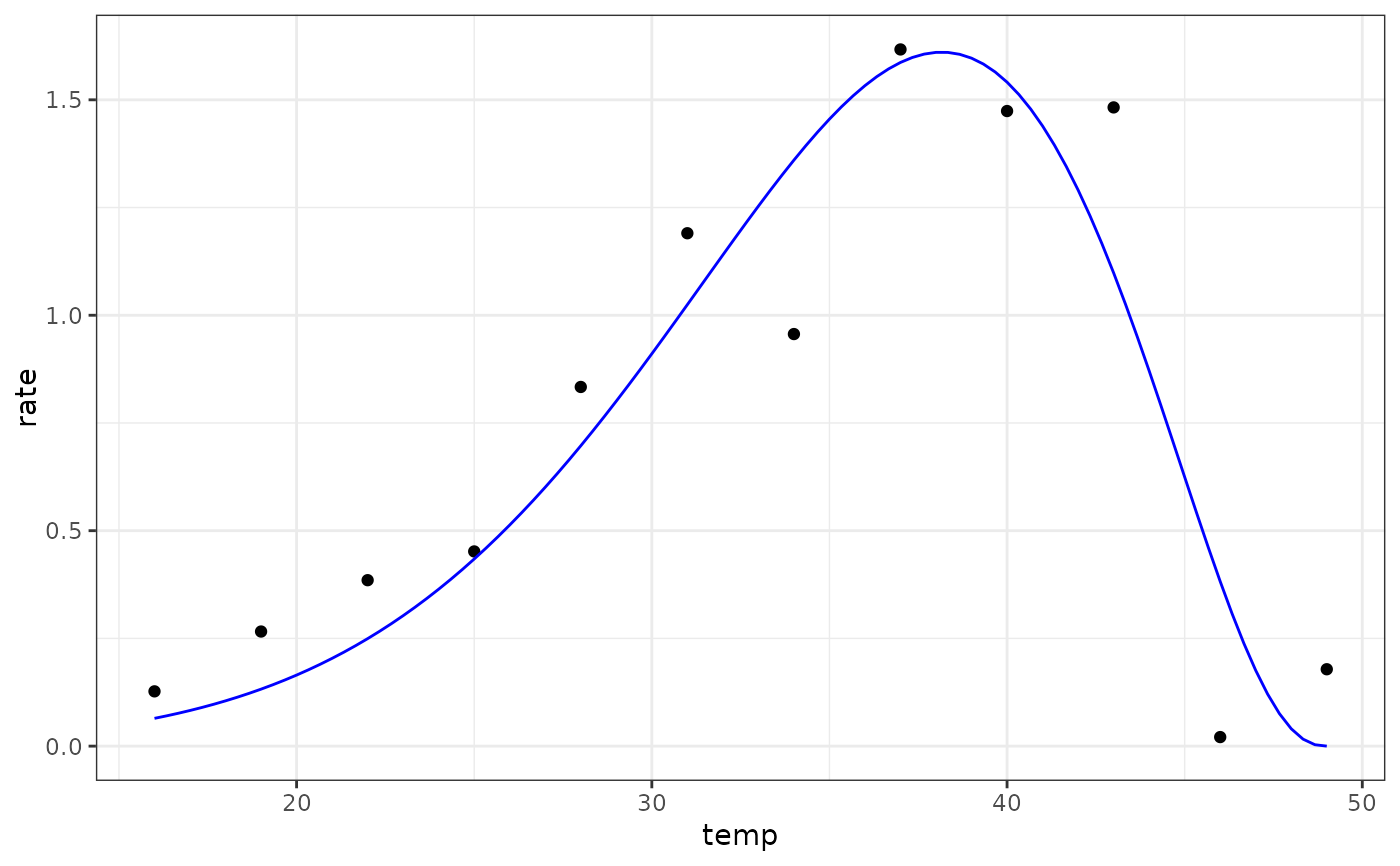
Extended Brière model for fitting thermal performance curves

Usage

briereextended_2021(temp, tmin, tmax, a, b, d)

Arguments

temp: temperature in degrees centigrade
tmin: low temperature (ºC) at which rates become negative
tmax: high temperature (ºC) at which rates become negative
a: scale parameter to adjust maximum rate of the curve
b: shape parameter to adjust the asymmetry of the curve
d: shape parameter to adjust the asymmetry of the curve

Value

a numeric vector of rate values based on the temperatures and parameter values provided to the function

Details

Equation: $$rate=a \cdot temp \cdot (temp - t_{min})^b \cdot (t_{max} - temp)^d$$

Start values in get_start_vals are derived from the data or sensible values from the literature.

Limits in get_lower_lims and get_upper_lims are derived from the data or based extreme values that are unlikely to occur in ecological settings.

Note

Generally we found this model easy to fit.

References

Cruz-Loya, M. et al. Antibiotics shift the temperature response curve of Escherichia coli growth. mSystems 6, e00228–21 (2021).

Examples

# load in ggplot
library(ggplot2)

# subset for the first TPC curve
data('chlorella_tpc')
d <- subset(chlorella_tpc, curve_id == 1)

# get start values and fit model
start_vals <- get_start_vals(d$temp, d$rate, model_name = 'briereextended_2021')
# fit model
mod <- nls.multstart::nls_multstart(rate~briereextended_2021(temp = temp, tmin, tmax, a, b, d),
data = d,
iter = c(4,4,4,4,4),
start_lower = start_vals - 10,
start_upper = start_vals + 10,
lower = get_lower_lims(d$temp, d$rate, model_name = 'briereextended_2021'),
upper = get_upper_lims(d$temp, d$rate, model_name = 'briereextended_2021'),
supp_errors = 'Y',
convergence_count = FALSE)

# look at model fit
summary(mod)
#> 
#> Formula: rate ~ briereextended_2021(temp = temp, tmin, tmax, a, b, d)
#> 
#> Parameters:
#>        Estimate Std. Error t value Pr(>|t|)   
#> tmin -4.728e+01  7.734e+02  -0.061  0.95296   
#> tmax  4.900e+01  1.057e+01   4.634  0.00239 **
#> a     5.624e-37  5.821e-34   0.001  0.99926   
#> b     1.676e+01  1.942e+02   0.086  0.93361   
#> d     2.411e+00  7.873e+00   0.306  0.76836   
#> ---
#> Signif. codes:  0 ‘***’ 0.001 ‘**’ 0.01 ‘*’ 0.05 ‘.’ 0.1 ‘ ’ 1
#> 
#> Residual standard error: 0.2841 on 7 degrees of freedom
#> 
#> Number of iterations to convergence: 57 
#> Achieved convergence tolerance: 1.49e-08
#> 

# get predictions
preds <- data.frame(temp = seq(min(d$temp), max(d$temp), length.out = 100))
preds <- broom::augment(mod, newdata = preds)

# plot
ggplot(preds) +
geom_point(aes(temp, rate), d) +
geom_line(aes(temp, .fitted), col = 'blue') +
theme_bw()