DeLong enzyme-assisted Arrhenius model for fitting thermal performance curves

Usage

delong_2017(temp, c, eb, ef, tm, ehc)

Arguments

temp: temperature in degrees centigrade
c: potential reaction rate
eb: baseline energy needed for the reaction to occur (eV)
ef: temperature dependence of folding the enzymes used in the metabolic reaction, relative to the melting temperature (eV)
tm: melting temperature in degrees centigrade
ehc: temperature dependence of the heat capacity between the folded and unfolded state of the enzymes, relative to the melting temperature (eV)

Value

a numeric vector of rate values based on the temperatures and parameter values provided to the function

Details

Equation: $$rate = c \cdot exp\frac{-(e_b-(e_f(1-\frac{temp + 273.15}{t_m})+e_{hc} \cdot ((temp + 273.15) - t_m - (temp + 273.15) \cdot ln(\frac{temp + 273.15}{t_m}))))}{k \cdot (temp + 273.15)}$$

where k is Boltzmann's constant with a value of 8.62e-05 and tm is actually tm - 273.15

Start values in get_start_vals are derived from the data or sensible values from the literature.

Limits in get_lower_lims and get_upper_lims are derived from the data or based extreme values that are unlikely to occur in ecological settings.

Note

Generally we found this model easy to fit.

References

DeLong, John P., et al. The combined effects of reactant kinetics and enzyme stability explain the temperature dependence of metabolic rates. Ecology and evolution 7.11 (2017): 3940-3950.

Examples

# load in ggplot
library(ggplot2)

# subset for the first TPC curve
data('chlorella_tpc')
d <- subset(chlorella_tpc, curve_id == 1)

# get start values and fit model
start_vals <- get_start_vals(d$temp, d$rate, model_name = 'delong_2017')
# fit model
mod <- nls.multstart::nls_multstart(rate~delong_2017(temp = temp, c, eb, ef, tm,ehc),
data = d,
iter = c(4,4,4,4,4),
start_lower = start_vals - 10,
start_upper = start_vals + 10,
lower = get_lower_lims(d$temp, d$rate, model_name = 'delong_2017'),
upper = get_upper_lims(d$temp, d$rate, model_name = 'delong_2017'),
supp_errors = 'Y',
convergence_count = FALSE)

# look at model fit
summary(mod)
#> 
#> Formula: rate ~ delong_2017(temp = temp, c, eb, ef, tm, ehc)
#> 
#> Parameters:
#>      Estimate Std. Error t value Pr(>|t|)  
#> c   7.225e+03  1.089e+11   0.000   1.0000  
#> eb  2.264e-01  4.025e+05   0.000   1.0000  
#> ef  2.602e-01  4.492e+05   0.000   1.0000  
#> tm  3.639e+01  6.823e+05   0.000   1.0000  
#> ehc 1.575e-01  5.906e-02   2.667   0.0321 *
#> ---
#> Signif. codes:  0 ‘***’ 0.001 ‘**’ 0.01 ‘*’ 0.05 ‘.’ 0.1 ‘ ’ 1
#> 
#> Residual standard error: 0.3787 on 7 degrees of freedom
#> 
#> Number of iterations to convergence: 44 
#> Achieved convergence tolerance: 1.49e-08
#> 

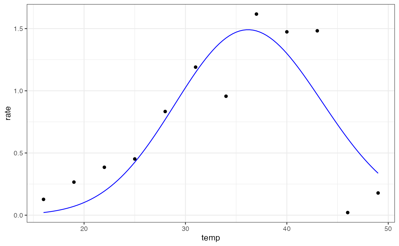
# get predictions
preds <- data.frame(temp = seq(min(d$temp), max(d$temp), length.out = 100))
preds <- broom::augment(mod, newdata = preds)

# plot
ggplot(preds) +
geom_point(aes(temp, rate), d) +
geom_line(aes(temp, .fitted), col = 'blue') +
theme_bw()