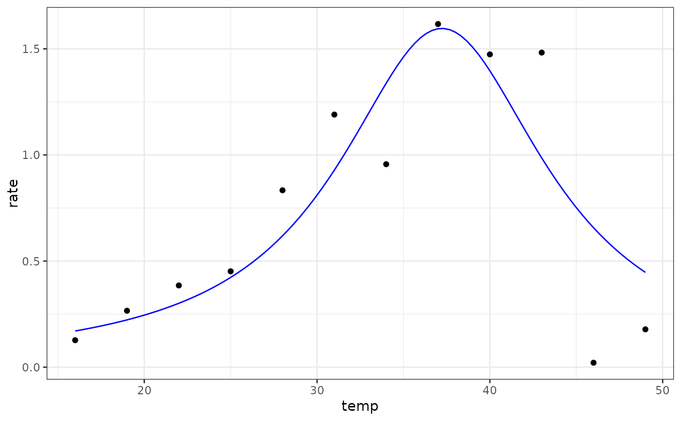
Eubank model for fitting thermal performance curves
Value
a numeric vector of rate values based on the temperatures and parameter values provided to the function
Details
Equation: $$rate = \frac{a}{(T-T_{\text{opt}})^2+b}$$
Start values in get_start_vals are derived from the data or sensible values from the literature.
Limits in get_lower_lims and get_upper_lims are based on extreme values that are unlikely to occur in ecological settings.
References
Eubank, W. P., Atmar, J. W. & Ellington, J. J. The significance and thermodynamics of fluctuating versus static thermal environments on Heliothis zea egg development rates. Environ. Entomol. 2, 491–496 (1973).
Examples
# load in ggplot
library(ggplot2)

# subset for the first TPC curve
data('chlorella_tpc')
d <- subset(chlorella_tpc, curve_id == 1)

# get start values and fit model
start_vals <- get_start_vals(d$temp, d$rate, model_name = 'eubank_1973')
# fit model
mod <- nls.multstart::nls_multstart(rate~eubank_1973(temp = temp, topt, a, b),
data = d,
iter = 200,
start_lower = start_vals - 10,
start_upper = start_vals + 10,
lower = get_lower_lims(d$temp, d$rate, model_name = 'eubank_1973'),
upper = get_upper_lims(d$temp, d$rate, model_name = 'eubank_1973'),
supp_errors = 'Y',
convergence_count = FALSE)

# look at model fit
summary(mod)
#>
#> Formula: rate ~ eubank_1973(temp = temp, topt, a, b)
#>
#> Parameters:
#>      Estimate Std. Error t value Pr(>|t|)
#> topt   37.225      1.124  33.124 1.03e-10 ***
#> a      86.015     33.164   2.594   0.0290 *
#> b      53.887     25.864   2.084   0.0669 .
#> ---
#> Signif. codes:  0 ‘***’ 0.001 ‘**’ 0.01 ‘*’ 0.05 ‘.’ 0.1 ‘ ’ 1
#>
#> Residual standard error: 0.3336 on 9 degrees of freedom
#>
#> Number of iterations to convergence: 24
#> Achieved convergence tolerance: 1.49e-08
#>

# get predictions
preds <- data.frame(temp = seq(min(d$temp), max(d$temp), length.out = 100))
preds <- broom::augment(mod, newdata = preds)

# plot
ggplot(preds) +
geom_point(aes(temp, rate), d) +
geom_line(aes(temp, .fitted), col = 'blue') +
theme_bw()

