Gaussian model for fitting thermal performance curves
Value
a numeric vector of rate values based on the temperatures and parameter values provided to the function
Details
Equation: $$rate = r_{max} \cdot exp^{\bigg(-0.5 \left(\frac{|temp-t_{opt}|}{a}\right)^2\bigg)}$$
Start values in get_start_vals are derived from the data
Limits in get_lower_lims and get_upper_lims are based on extreme values that are unlikely to occur in ecological settings.
References
Lynch, M., Gabriel, W., Environmental tolerance. The American Naturalist. 129, 283–303. (1987)
Examples
# load in ggplot
library(ggplot2)
# subset for the first TPC curve
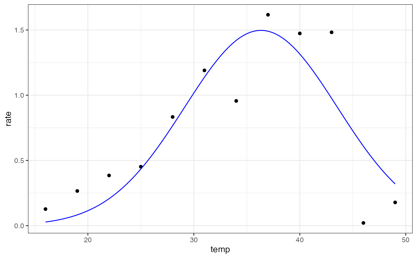
data('chlorella_tpc')
d <- subset(chlorella_tpc, curve_id == 1)
# get start values and fit model
start_vals <- get_start_vals(d$temp, d$rate, model_name = 'gaussian_1987')
# fit model
mod <- nls.multstart::nls_multstart(rate~gaussian_1987(temp = temp,rmax, topt,a),
data = d,
iter = c(4,4,4),
start_lower = start_vals - 10,
start_upper = start_vals + 10,
lower = get_lower_lims(d$temp, d$rate, model_name = 'gaussian_1987'),
upper = get_upper_lims(d$temp, d$rate, model_name = 'gaussian_1987'),
supp_errors = 'Y',
convergence_count = FALSE)
# look at model fit
summary(mod)
#>
#> Formula: rate ~ gaussian_1987(temp = temp, rmax, topt, a)
#>
#> Parameters:
#> Estimate Std. Error t value Pr(>|t|)
#> rmax 1.4972 0.1963 7.627 3.23e-05 ***
#> topt 36.3381 1.0928 33.253 9.91e-11 ***
#> a 7.2062 1.1396 6.323 0.000137 ***
#> ---
#> Signif. codes: 0 ‘***’ 0.001 ‘**’ 0.01 ‘*’ 0.05 ‘.’ 0.1 ‘ ’ 1
#>
#> Residual standard error: 0.3268 on 9 degrees of freedom
#>
#> Number of iterations to convergence: 20
#> Achieved convergence tolerance: 1.49e-08
#>
# get predictions
preds <- data.frame(temp = seq(min(d$temp), max(d$temp), length.out = 100))
preds <- broom::augment(mod, newdata = preds)
# plot
ggplot(preds) +
geom_point(aes(temp, rate), d) +
geom_line(aes(temp, .fitted), col = 'blue') +
theme_bw()