Modified gaussian model for fitting thermal performance curves

Usage

gaussianmodified_2006(temp, rmax, topt, a, b)

Arguments

temp: temperature in degrees centigrade
rmax: maximum rate at optimum temperature
topt: optimum temperature
a: related to full curve width
b: allows for asymmetry in the curve fit

Value

a numeric vector of rate values based on the temperatures and parameter values provided to the function

Details

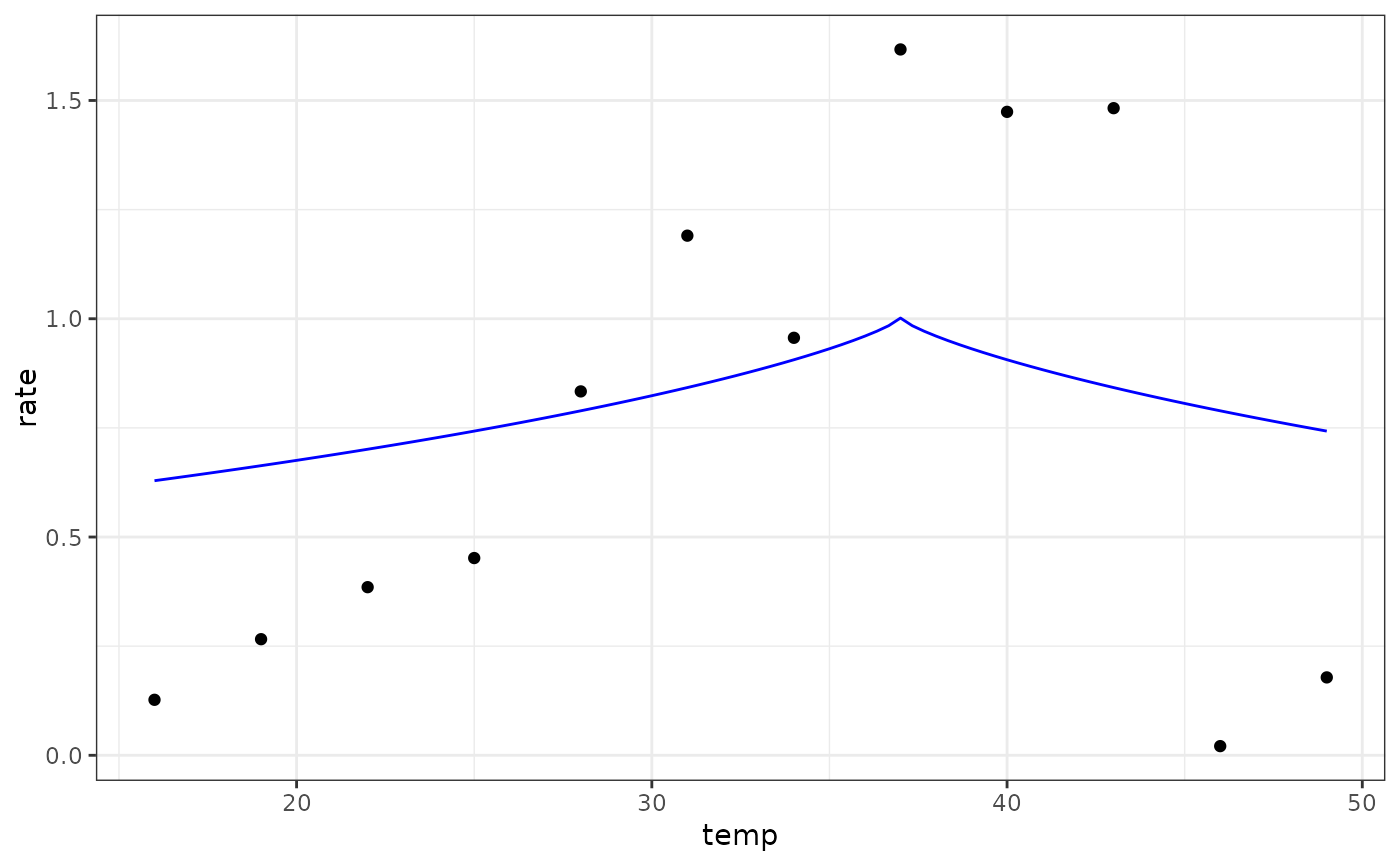
Equation: $$rate = r_{max} \cdot \exp{\bigg[-0.5 \left(\frac{|temp-t_{opt}|}{a}\right)^b\bigg]}$$

Start values in get_start_vals are derived from the data and gaussian_1987

Limits in get_lower_lims and get_upper_lims are based on extreme values that are unlikely to occur in ecological settings.

Note

Generally we found this model difficult to fit.

This function was previously called modifiedgaussian_2006() however this is now deprecated and will be removed in the future.

References

Angilletta Jr, M. J. (2006). Estimating and comparing thermal performance curves. Journal of Thermal Biology, 31(7), 541-545.

Examples

# load in ggplot
library(ggplot2)

# subset for the first TPC curve
data('chlorella_tpc')
d <- subset(chlorella_tpc, curve_id == 1)

# get start values and fit model
start_vals <- get_start_vals(d$temp, d$rate, model_name = 'gaussianmodified_2006')
# fit model
mod <- nls.multstart::nls_multstart(rate~gaussianmodified_2006(temp = temp, rmax, topt, a, b),
data = d,
iter = c(3,3,3,3),
start_lower = start_vals - 10,
start_upper = start_vals + 10,
lower = get_lower_lims(d$temp, d$rate, model_name = 'gaussianmodified_2006'),
upper = get_upper_lims(d$temp, d$rate, model_name = 'gaussianmodified_2006'),
supp_errors = 'Y',
convergence_count = FALSE)

# look at model fit
summary(mod)
#> 
#> Formula: rate ~ gaussianmodified_2006(temp = temp, rmax, topt, a, b)
#> 
#> Parameters:
#>      Estimate Std. Error t value Pr(>|t|)    
#> rmax   1.0016     2.0083   0.499    0.631    
#> topt  37.0000     2.7728  13.344 9.51e-07 ***
#> a     23.0120    90.9028   0.253    0.807    
#> b      0.7888     7.1214   0.111    0.915    
#> ---
#> Signif. codes:  0 ‘***’ 0.001 ‘**’ 0.01 ‘*’ 0.05 ‘.’ 0.1 ‘ ’ 1
#> 
#> Residual standard error: 0.5851 on 8 degrees of freedom
#> 
#> Number of iterations to convergence: 20 
#> Achieved convergence tolerance: 1.49e-08
#> 

# get predictions
preds <- data.frame(temp = seq(min(d$temp), max(d$temp), length.out = 100))
preds <- broom::augment(mod, newdata = preds)

# plot
ggplot(preds) +
geom_point(aes(temp, rate), d) +
geom_line(aes(temp, .fitted), col = 'blue') +
theme_bw()