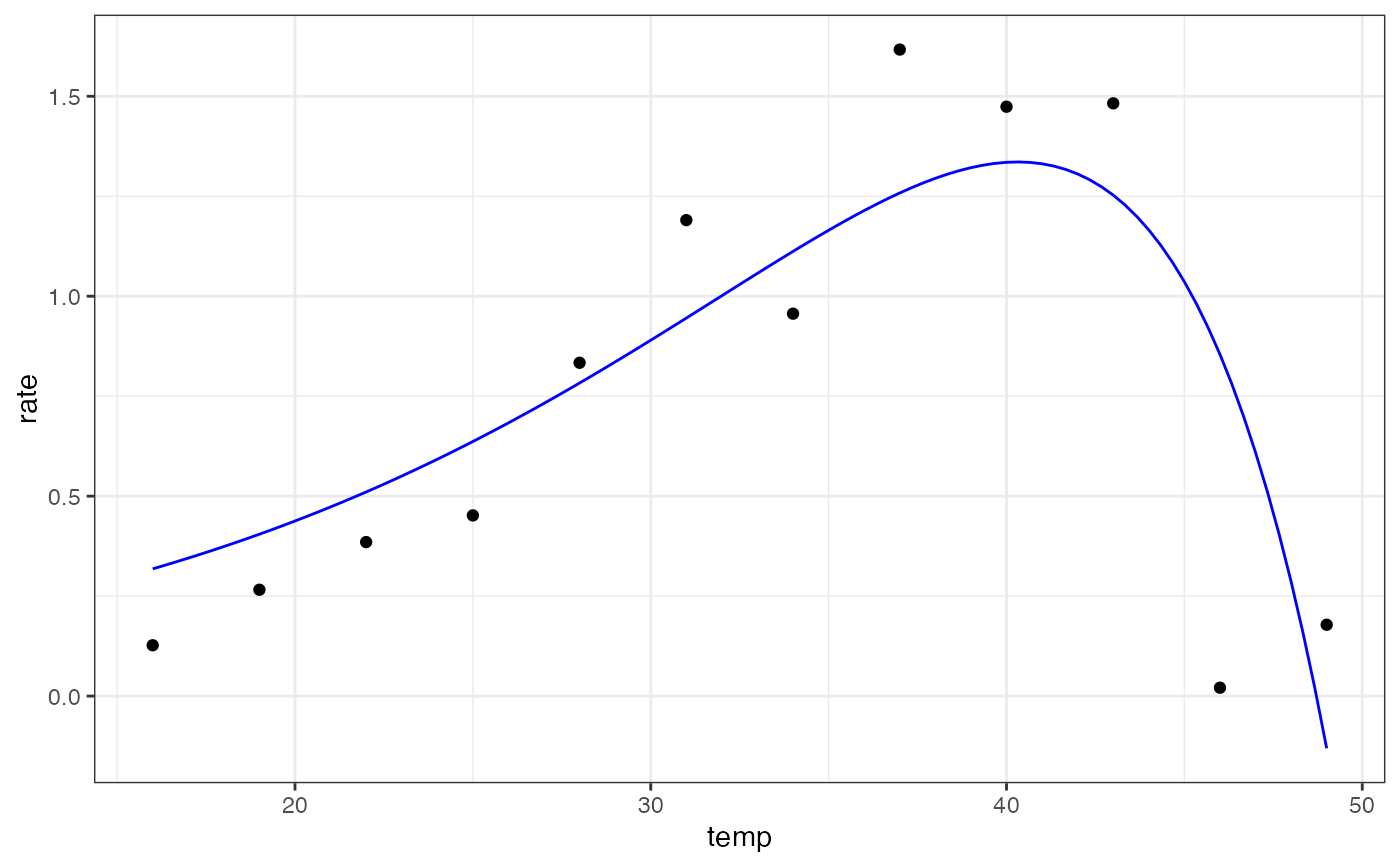
Hinshelwood model for fitting thermal performance curves

Usage

hinshelwood_1947(temp, a, e, b, eh)

Arguments

temp: temperature in degrees centigrade
a: pre-exponential constant for the activation energy
e: activation energy (eV)
b: pre-exponential constant for the deactivation energy
eh: de-activation energy (eV)

Value

a numeric vector of rate values based on the temperatures and parameter values provided to the function

Details

Equation: $$rate=a \cdot exp^{\frac{-e}{k \cdot (temp + 273.15)}} - b \cdot exp^\frac{-e_h}{k \cdot (temp + 273.15)}$$

where k is Boltzmann's constant with a value of 8.62e-05

Start values in get_start_vals are taken from the literature.

Limits in get_lower_lims and get_upper_lims are based on extreme values that are unlikely to occur in ecological settings.

Note

Generally we found this model difficult to fit.

References

Hinshelwood C.N. The Chemical Kinetics of the Bacterial Cell. Oxford University Press. (1947)

Examples

# load in ggplot
library(ggplot2)

# subset for the first TPC curve
data('chlorella_tpc')
d <- subset(chlorella_tpc, curve_id == 1)

# get start values and fit model
start_vals <- get_start_vals(d$temp, d$rate, model_name = 'hinshelwood_1947')
# fit model
mod <- nls.multstart::nls_multstart(rate~hinshelwood_1947(temp = temp,a, e, b, eh),
data = d,
iter = c(5,5,5,5),
start_lower = start_vals - 1,
start_upper = start_vals + 1,
lower = get_lower_lims(d$temp, d$rate, model_name = 'hinshelwood_1947'),
upper = get_upper_lims(d$temp, d$rate, model_name = 'hinshelwood_1947'),
supp_errors = 'Y',
convergence_count = FALSE)

# look at model fit
summary(mod)
#> 
#> Formula: rate ~ hinshelwood_1947(temp = temp, a, e, b, eh)
#> 
#> Parameters:
#>     Estimate Std. Error t value Pr(>|t|)
#> a  1.104e+10  2.530e+11   0.044    0.966
#> e  6.045e-01  5.823e-01   1.038    0.330
#> b  1.479e+26  9.735e+27   0.015    0.988
#> eh 1.635e+00  1.878e+00   0.870    0.409
#> 
#> Residual standard error: 0.3846 on 8 degrees of freedom
#> 
#> Number of iterations till stop: 96 
#> Achieved convergence tolerance: 1.49e-08
#> Reason stopped: Number of calls to `fcn' has reached or exceeded `maxfev' == 500.
#> 

# get predictions
preds <- data.frame(temp = seq(min(d$temp), max(d$temp), length.out = 100))
preds <- broom::augment(mod, newdata = preds)

# plot
ggplot(preds) +
geom_point(aes(temp, rate), d) +
geom_line(aes(temp, .fitted), col = 'blue') +
theme_bw()