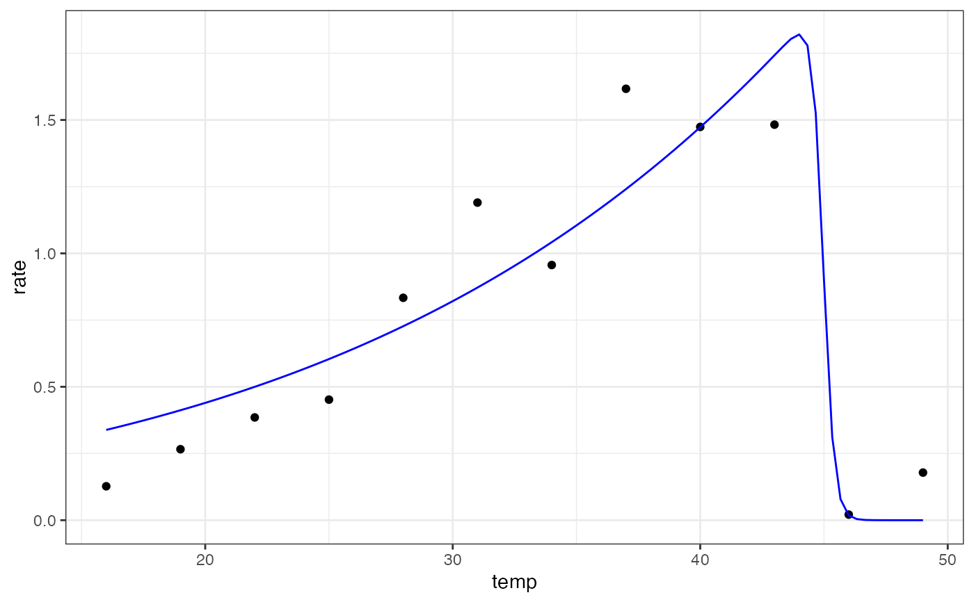
Johnson-Lewin model for fitting thermal performance curves

Usage

johnsonlewin_1946(temp, r0, e, eh, topt)

Arguments

temp: temperature in degrees centigrade
r0: scaling parameter
e: activation energy (eV)
eh: high temperature de-activation energy (eV)
topt: optimum temperature (ºC)

Value

a numeric vector of rate values based on the temperatures and parameter values provided to the function

Details

Equation: $$rate= \frac{r_0 \cdot exp^{\frac{-e}{k\cdot (temp + 273.15)}}}{1 + exp^{-\frac{e_h -\big(\frac{e_h}{(t_{opt} + 273.15)} + k \cdot ln\big(\frac{e}{e_h - e}\big) \big) \cdot (temp + 273.15)}{k \cdot (temp + 273.15)}}}$$

where k is Boltzmann's constant with a value of 8.62e-05.

Start values in get_start_vals are derived from the data.

Limits in get_lower_lims and get_upper_lims are derived from the data or based extreme values that are unlikely to occur in ecological settings.

Note

Generally we found this model difficult to fit.

References

Johnson, Frank H., and Isaac Lewin. The growth rate of E. coli in relation to temperature, quinine and coenzyme. Journal of Cellular and Comparative Physiology 28.1 (1946): 47-75.

Examples

# \donttest{
# load in ggplot
library(ggplot2)

# subset for the first TPC curve
data('chlorella_tpc')
d <- subset(chlorella_tpc, curve_id == 1)

# get start values and fit model
start_vals <- get_start_vals(d$temp, d$rate, model_name = 'johnsonlewin_1946')
# fit model
mod <- suppressWarnings(
nls.multstart::nls_multstart(rate~johnsonlewin_1946(temp = temp, r0, e, eh, topt),
data = d,
iter = c(5,5,5,5),
start_lower = start_vals - 1,
start_upper = start_vals + 1,
lower = get_lower_lims(d$temp, d$rate, model_name = 'johnsonlewin_1946'),
upper = get_upper_lims(d$temp, d$rate, model_name = 'johnsonlewin_1946'),
supp_errors = 'Y',
convergence_count = FALSE)
)

# look at model fit
summary(mod)
#> 
#> Formula: rate ~ johnsonlewin_1946(temp = temp, r0, e, eh, topt)
#> 
#> Parameters:
#>       Estimate Std. Error t value Pr(>|t|)   
#> r0   7.322e+07  3.295e+08   0.222  0.82968   
#> e    4.784e-01  1.191e-01   4.016  0.00386 **
#> eh   4.000e+01  5.278e+03   0.008  0.99414   
#> topt 4.401e+01  2.324e+02   0.189  0.85453   
#> ---
#> Signif. codes:  0 ‘***’ 0.001 ‘**’ 0.01 ‘*’ 0.05 ‘.’ 0.1 ‘ ’ 1
#> 
#> Residual standard error: 0.2406 on 8 degrees of freedom
#> 
#> Number of iterations till stop: 97 
#> Achieved convergence tolerance: 1.49e-08
#> Reason stopped: Number of calls to `fcn' has reached or exceeded `maxfev' == 500.
#> 

# get predictions
preds <- data.frame(temp = seq(min(d$temp), max(d$temp), length.out = 100))
preds <- broom::augment(mod, newdata = preds)

# plot
ggplot(preds) +
geom_point(aes(temp, rate), d) +
geom_line(aes(temp, .fitted), col = 'blue') +
theme_bw()

# }