Mitchell Angilletta model for fitting thermal performance curves

Usage

mitchell_2009(temp, topt, a, b)

Arguments

temp: temperature in degrees centigrade
topt: optimum temperature (ºC) where rate is maximal
a: scale parameter to convert the value of the cosine density to the appropriate magnitude
b: parameter dictating the performance breadth

Value

a numeric vector of rate values based on the temperatures and parameter values provided to the function

Details

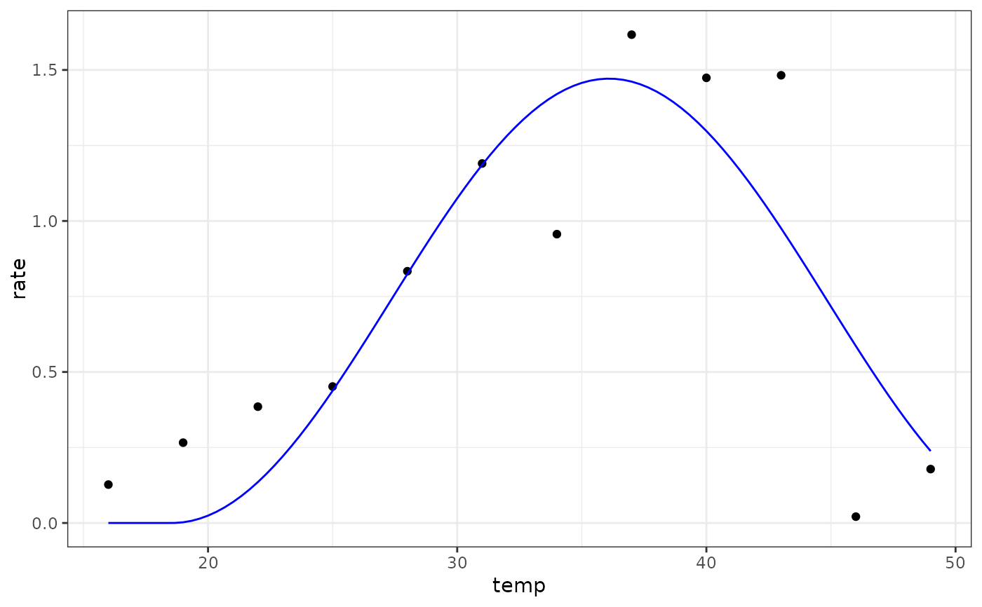
Equation: $$rate=\frac{1}{2 \cdot b} \cdot (1 + cos(\frac{temp - t_{opt}}{b} \cdot \pi)) \cdot a $$

When temperatures fall below topt - b or above topt + b, rates are set to 0 to prevent multimodality.

Start values in get_start_vals are derived from the data or sensible values from the literature.

Limits in get_lower_lims and get_upper_lims are derived from the data or based extreme values that are unlikely to occur in ecological settings.

Note

Generally we found this model easy to fit.

References

Mitchell, W. A., & Angilletta Jr, M. J. (2009). Thermal games: frequency-dependent models of thermal adaptation. Functional Ecology, 510-520.

Author

Daniel Padfield

Examples

# load in ggplot
library(ggplot2)

# subset for the first TPC curve
data('chlorella_tpc')
d <- subset(chlorella_tpc, curve_id == 1)

# get start values and fit model
start_vals <- get_start_vals(d$temp, d$rate, model_name = 'mitchell_2009')
# fit model
mod <- nls.multstart::nls_multstart(rate~mitchell_2009(temp = temp, topt, a, b),
data = d,
iter = c(3,3,3),
start_lower = start_vals - 10,
start_upper = start_vals + 10,
lower = get_lower_lims(d$temp, d$rate, model_name = 'mitchell_2009'),
upper = get_upper_lims(d$temp, d$rate, model_name = 'mitchell_2009'),
supp_errors = 'Y',
convergence_count = FALSE)

# look at model fit
summary(mod)
#> 
#> Formula: rate ~ mitchell_2009(temp = temp, topt, a, b)
#> 
#> Parameters:
#>      Estimate Std. Error t value Pr(>|t|)    
#> topt   36.090      1.053  34.275 7.56e-11 ***
#> a      25.789      3.291   7.837 2.61e-05 ***
#> b      17.530      2.366   7.410 4.06e-05 ***
#> ---
#> Signif. codes:  0 ‘***’ 0.001 ‘**’ 0.01 ‘*’ 0.05 ‘.’ 0.1 ‘ ’ 1
#> 
#> Residual standard error: 0.333 on 9 degrees of freedom
#> 
#> Number of iterations to convergence: 38 
#> Achieved convergence tolerance: 1.49e-08
#> 

# get predictions
preds <- data.frame(temp = seq(min(d$temp), max(d$temp), length.out = 100))
preds <- broom::augment(mod, newdata = preds)

# plot
ggplot(preds) +
geom_point(aes(temp, rate), d) +
geom_line(aes(temp, .fitted), col = 'blue') +
theme_bw()