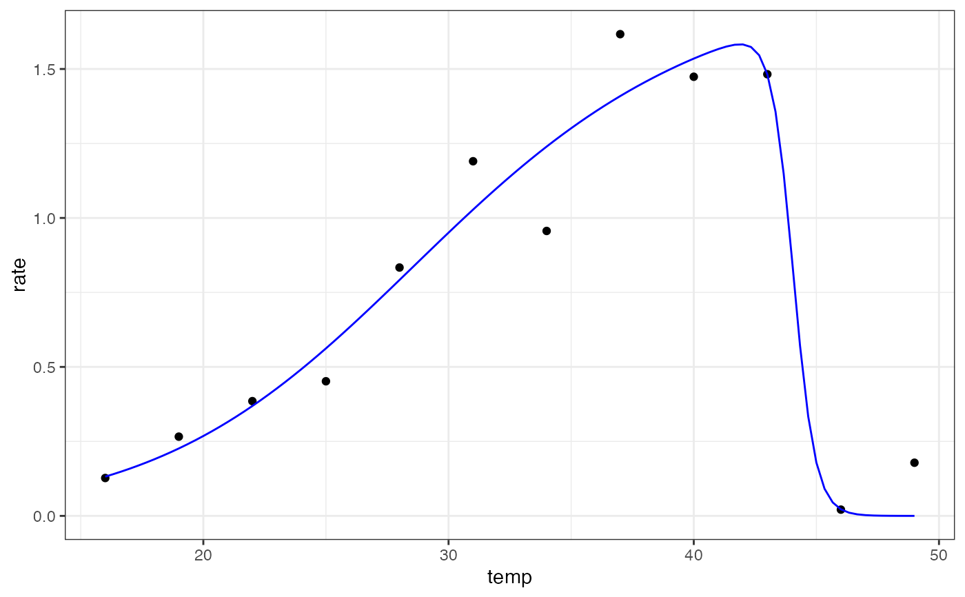
Full Sharpe-Schoolfield model for fitting thermal performance curves

Usage

sharpeschoolfull_1981(temp, r_tref, e, el, tl, eh, th, tref)

Arguments

temp: temperature in degrees centigrade
r_tref: rate at the standardised temperature, tref
e: activation energy (eV)
el: low temperature de-activation energy (eV)
tl: temperature (ºC) at which enzyme is 1/2 active and 1/2 suppressed due to low temperatures
eh: high temperature de-activation energy (eV)
th: temperature (ºC) at which enzyme is 1/2 active and 1/2 suppressed due to high temperatures
tref: standardisation temperature in degrees centigrade. Temperature at which rates are not inactivated by either high or low temperatures

Value

a numeric vector of rate values based on the temperatures and parameter values provided to the function

Details

Equation: $$rate= \frac{r_{tref} \cdot exp^{\frac{-e}{k} (\frac{1}{temp + 273.15}-\frac{1}{t_{ref} + 273.15})}}{1+ exp^{\frac{e_l}{k}(\frac{1}{t_l} - \frac{1}{temp + 273.15})} + exp^{\frac{e_h}{k}(\frac{1}{t_h}-\frac{1}{temp + 273.15})}}$$

where k is Boltzmann's constant with a value of 8.62e-05.

Start values in get_start_vals are derived from the data.

Limits in get_lower_lims and get_upper_lims are derived from the data or based extreme values that are unlikely to occur in ecological settings.

Note

Generally we found this model easy to fit.

References

Schoolfield, R. M., Sharpe, P. J. & Magnuson, C. E. Non-linear regression of biological temperature-dependent rate models based on absolute reaction-rate theory. Journal of Theoretical Biology 88, 719-731 (1981)

Author

Daniel Padfield

Examples

# load in ggplot
library(ggplot2)
library(nls.multstart)

# subset for the first TPC curve
data('chlorella_tpc')
d <- subset(chlorella_tpc, curve_id == 1)

# get start values and fit model
start_vals <- get_start_vals(d$temp, d$rate, model_name = 'sharpeschoolfull_1981')
# fit model
mod <- nls_multstart(rate~sharpeschoolfull_1981(temp = temp, r_tref, e, el, tl, eh, th, tref = 20),
data = d,
iter = c(3,3,3,3,3,3),
start_lower = start_vals - 10,
start_upper = start_vals + 10,
lower = get_lower_lims(d$temp, d$rate, model_name = 'sharpeschoolfull_1981'),
upper = get_upper_lims(d$temp, d$rate, model_name = 'sharpeschoolfull_1981'),
supp_errors = 'Y',
convergence_count = FALSE)

# look at model fit
summary(mod)
#> 
#> Formula: rate ~ sharpeschoolfull_1981(temp = temp, r_tref, e, el, tl, 
#>     eh, th, tref = 20)
#> 
#> Parameters:
#>        Estimate Std. Error t value Pr(>|t|)    
#> r_tref  1.61689    4.91089   0.329   0.7532    
#> e       0.02815    1.01715   0.028   0.9788    
#> el      1.44338    0.68857   2.096   0.0809 .  
#> tl     28.53344   21.51355   1.326   0.2330    
#> eh     19.24223   25.84740   0.744   0.4847    
#> th     44.01635    1.62323  27.116 1.66e-07 ***
#> ---
#> Signif. codes:  0 ‘***’ 0.001 ‘**’ 0.01 ‘*’ 0.05 ‘.’ 0.1 ‘ ’ 1
#> 
#> Residual standard error: 0.1831 on 6 degrees of freedom
#> 
#> Number of iterations to convergence: 47 
#> Achieved convergence tolerance: 1.49e-08
#> 

# get predictions
preds <- data.frame(temp = seq(min(d$temp), max(d$temp), length.out = 100))
preds <- broom::augment(mod, newdata = preds)

# plot
ggplot(preds) +
geom_point(aes(temp, rate), d) +
geom_line(aes(temp, .fitted), col = 'blue') +
theme_bw()